Some authors brag that their scanners are faster than Nmap because of stateless operation. They simply blast out a flood of packets then listen for responses and hope for the best. While this may have value for quick surveys and other cases where speed is more important than comprehensiveness and accuracy, I don't find it appropriate for security scanning. A stateless scanner cannot detect dropped packets in order to retransmit and throttle its send rate. If a busy router half way along the network path drops 80% of the scanner's packet flood, the scanner will still consider the run successful and print results that are woefully inaccurate. Nmap, on the other hand, saves extensive state in RAM while it runs. There is usually plenty of memory available, even on a PDA. Nmap marks each probe with sequence numbers, source or destination ports, ID fields, or other aspects (depending on probe type) which allow it to recognize responses (and thus drops). It then adjusts its speed appropriately to stay as fast as the network (and given command-line options) allow without crossing the line and suffering inaccuracy or unfairly hogging a shared network. Some administrators who have not installed an IDS might not notice an Nmap SYN scan of their whole network. But you better believe the administrator will investigate if you use a brute packet flooding scanner that affects his Quake ping time!

While Nmap's congestion control algorithms are recommended for most scans, they can be overridden. The --min-rate option sends packets at the rate you specify (or higher) even if that exceeds Nmap's normal congestion control limits. Similarly, the --max-retries option controls how many times Nmap may retransmit a packet. Options such as --min-rate 100 --max-retries 0 will emulate the behavior of simple stateless scanners. You could double that speed by specifying a rate of 200 packets per second rather than 100, but don't get too greedy—an extremely fast scan is of little value if the results are wrong or incomplete. Any use of --min-rate is at your own risk.

Most of the diagrams in this chapter illustrate the use of a technique to determine the state of a single port. Sending a probe and receiving the response takes at least one round trip time (RTT) between the source and target machines. If your RTT is 200 ms and you are scanning 65,536 ports on a machine, handling them serially would take at least 3.6 hours. Scan a network of 20,000 machines that way and the wait balloons to more than eight years. This is clearly unacceptable so Nmap parallelizes its scans and is capable of scanning hundreds of ports on each of dozens of machines at the same time. This improves speeds by several orders of magnitude. The number of hosts and ports it scans at a time is dependent on arguments described in Chapter 6, Optimizing Nmap Performance, including --min-hostgroup, --min-parallelism, -T4, --max-rtt-timeout, and many others. It also depends on network conditions detected by Nmap.

When scanning multiple machines, Nmap tries to efficiently spread the load between them. If a machine appears overwhelmed (drops packets or its latency increases), Nmap slows down for that host while continuing against others at full speed.

Every time a probe response is received, Nmap calculates the microseconds elapsed since the probe was sent. We'll call this the instanceRTT, and Nmap uses it to keep a running tally of three crucial timing-related values: srtt, rttvar, and timeout. Nmap keeps separate values for each host and also merged values for a whole group of hosts scanned in parallel. They are calculated as follows:

These simple time estimation formulas seem to work quite well. They are loosely based on similar techniques used by TCP and discussed in RFC 2988, Computing TCP's Retransmission Timer. We have optimized those algorithms over the years to better suit port scanning.

Retransmission timers are far from the only technique Nmap gleaned from TCP. Since Nmap is most commonly used with TCP, it is only fair to follow many of the same rules. Particularly since those rules are the result of substantial research into maximizing throughput without degrading into a tragedy of the commons where everyone selfishly hogs the network. With its default options, Nmap is reasonably polite. Nmap uses three algorithms modeled after TCP to control how aggressive the scan is: a congestion window, exponential backoff, and slow start. The congestion window controls how many probes Nmap may have outstanding at once. If the window is full, Nmap won't send any more until a response is received or a probe times out. Exponential backoff causes Nmap to slow down dramatically when it detects dropped packets. The congestion window is usually reduced to one whenever drops are detected. Despite slow being in the name, slow start is a rather quick algorithm for gradually increasing the scan speed to determine the performance limits of the network.

All of these techniques are described in RFC 2581, TCP Congestion Control. That document was written by networking gurus Richard Stevens, Vern Paxson, and Mark Allman. It is only 10 pages long and anyone interested in implementing efficient TCP stacks (or other network protocols, or port scanners) should find it fascinating.

When Nmap scans a group of targets, it maintains in memory a congestion window and threshold for each target, as well as a window and threshold for the group as a whole. The congestion window is the number of probes that may be sent at one time. The congestion threshold defines the boundary between slow start and congestion avoidance modes. During slow start, the congestion window grows rapidly in response to responses. Once the congestion window exceeds the congestion threshold, congestion avoidance mode begins, during which the congestion window increases more slowly. After a drop, both the congestion window and threshold are reduced to some fraction of their previous value.

There is an important difference between TCP streams and Nmap port scans, however. In TCP streams, it's normal to expect ACKs in response to every packet sent (or at least a large fraction of them). In fact, proper growth of the congestion window depends on this assumption. Nmap often finds itself in a different situation: facing a target with a default-deny firewall, very few sent packets will ever be responded to. The same thing happens when ping scanning a block of network addresses that contains only a few live hosts. To compensate for this, Nmap keeps track of the ratio of packets sent to responses received. Any time the group congestion window changes, the amount of the change is multiplied by this ratio. In other words, when few packets receive responses, each response carries more weight.

A graphical description of how the group congestion window and threshold vary during a typical port scan is shown in Figure 5.9. The congestion window is shown in black and the congestion threshold is in gray.

Figure 5.9. Congestion window and threshold

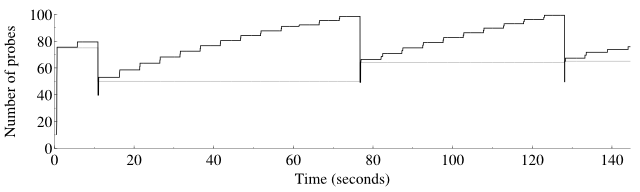
The congestion window starts low and the congestion threshold starts high. Slow start mode begins and the window size increases rapidly. The large “stairstep” jumps are the result of timing pings. At about 10 seconds, the congestion window has grown to 80 probes when a drop is detected. Both the congestion window and threshold are reduced. The congestion window continues to grow until about 80 seconds when another drop is detected. Then the cycle repeats, which is typical when network conditions are stable.

Drops during a scan are nothing to be afraid of. The purpose of the congestion control algorithms is to dynamically probe the network to discover its capacity. Viewed in this way, drops are valuable feedback that help Nmap determine the correct size for the congestion window.

Every technique discussed in this algorithms section involves (at some level) network monitoring to detect and estimate network packet loss and latency. This really is critical to obtaining fast scan times. Unfortunately, good data is often difficult to come by when scanning heavily firewalled systems. These filters often drop the overwhelming majority of packets without any response. Nmap may have to send 20,000 probes or more to find one responsive port, making it difficult to monitor network conditions.

To combat this problem, Nmap uses timing probes, also known as port scan pings. If Nmap has found at least one port responsive on a heavily filtered host, it will send a probe to that port every 1.25 seconds that it goes without receiving responses from any other ports. This allows Nmap to conduct a sufficient level of monitoring to speed up or slow down its scans as network conditions allow.

Sometimes even port scan pings won't help because no responsive ports at all have been found. The machine could be down (and scanned with -Pn), or every single port could be filtered. Or perhaps the target does have a couple responsive ports, but Nmap has not been lucky enough to find them yet. In these cases, Nmap uses timing values that it maintains for the whole group of machines it is scanning at the same time. As long as at least one response has been received from any machine in the group, Nmap has something to work with. Of course Nmap cannot assume that hosts in a group always share similar timing characteristics. So Nmap tracks the timing variances between responsive hosts in a group. If they differ wildly, Nmap infers long timeouts for neighboring hosts to be on the safe side.

The simplest of scanners (and the stateless ones) generally don't retransmit probes at all. They simply send a probe to each port and report based on the response or lack thereof. Slightly more complex scanners will retransmit a set number of times. Nmap tries to be smarter by keeping careful packet loss statistics for each scan against a target. If no packet loss is detected, Nmap may retransmit only once when it fails to receive a probe response. When massive packet loss is evident, Nmap may retransmit ten or more times. This allows Nmap to scan hosts on fast, reliable networks quickly, while preserving accuracy (at the expense of some speed) when scanning problematic networks or machines. Even Nmap's patience isn't unlimited though. At a certain point (ten retransmissions), Nmap will print a warning and give up on further retransmissions. This prevents malicious hosts from slowing Nmap down too much with intentional packet drops, slow responses, and similar shenanigans. That technique is known as tarpitting and is commonly used against spammers.

Packet response rate limiting is perhaps the most pernicious problem faced by port scanners such as Nmap. For example, Linux 2.4 kernels limit ICMP error messages returned during a UDP (-sU) or IP protocol (-sO) scan to one per second. If Nmap counted these as normal drops, it would be continually slowing down (remember exponential backoff) but still end up having the vast majority of its probes dropped. Instead, Nmap tries to detect this situation. When a large proportion of packets are being dropped, it implements a short delay (as little as 5 milliseconds) between each probe sent to a single target. 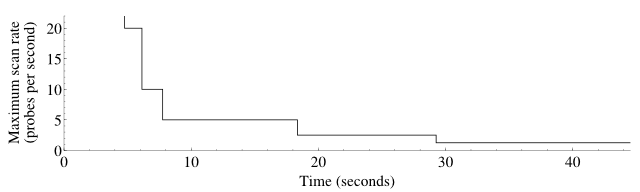If drops continue to be a major problem, Nmap will keep doubling the delay until the drops cease or Nmap hits the maximum allowed scan delay. The effects of scan delay while UDP scanning ports 1–50 of a response rate-limited Linux host are shown in Figure 5.10. At the beginning, the scan rate is unlimited by scan delay, though of course other mechanisms such as congestion control impose their own limits. When drops are detected, the scan delay is doubled, meaning that the maximum scan rate is effectively halved. In the graph, for example, a maximum scan rate of five packets per second corresponds to a scan delay of 200 milliseconds.

Figure 5.10. Scan rate as affected by scan delay

The maximum scan delay defaults to one second between probes. The scan delay is sometimes enabled when a slow host can't keep up, even when that host has no explicit rate limiting rules. This can reduce total network traffic substantially by reducing wasted (dropped) probe packets. Unfortunately even small scan delay values can make a scan takes several times as long. Nmap is conservative by default, allowing second-long scan delays for TCP and UDP probes. If your priorities differ, you can configure maximum scan delays with --max-scan-delay as discussed in Chapter 5, Port Scanning Techniques and Algorithms.